Load in relevant Packages.

library(tidycensus)
library(tidyverse)
library(tigris)
library(sf)
library(crsuggest)
library(patchwork)
library(units)
library(car)
library(spdep)
options(tigris_use_cache = TRUE)

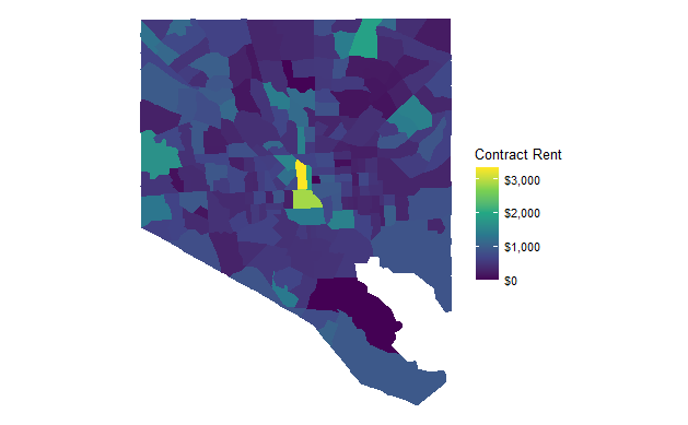
Obtain data on contract rent (variable B25056_001) for tracts in Baltimore City, with geometry.

balt_rent <- get_acs(
  geography = "tract", 
  variables = "B25056_001",
  state = "MD", 
  county = "Baltimore City",
  geometry = TRUE
)

Create a chloropleth map of average rent in each tract.

 ggplot(balt_rent, aes(fill = estimate)) + 
  geom_sf(color = NA) + 
  scale_fill_viridis_c(labels = scales::dollar) + 
  theme_void() + 
  labs(fill = "Contract Rent")

Get point data on serious (‘Part 1’) crimes from the Baltimore City website. Keep only the same time period as the 5-year ACS rent estimates (2015-2019).

crimedata<-read_sf(dsn = "C:/Users/rache/OneDrive/Documents/Advanced GIS Mahmoudi/Project1/Part1_Crime_data.shp", layer = "Part1_Crime_data")

crime_lowercutoff <- filter(crimedata, (crimedata$CrimeDateT >= "2015-01-01"))
crime_finalcutoff<- filter(lowercutoff, (lowercutoff$CrimeDateT< "2019-01-01"))

Transform both files to an appropriate coordinate reference system. Join the rent data with the crimes point data. Use the new file to obtain crime counts for each tract. Join this count file back to the original transformed rent shapefile.

#suggest_crs(crime_finalcutoff)
#suggestion was 32622

crimepoints_tr<-st_transform(crime_finalcutoff, 32622)
rent_tr<-st_transform(balt_rent, 32622)

crimesandrent_join <- st_join(crimepoints_tr, rent_tr, join = st_within)

crimecountbytract <- count(as_tibble(crimesandrent_join), GEOID)

alldatajoined_simple<- merge(rent_tr,crimecountbytract, by="GEOID")

Analysis With Simple Crime Counts

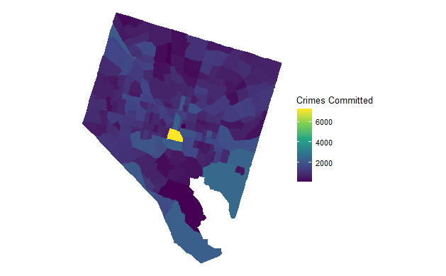
Create a chloropleth map of the number of crimes committed within each tract.

ggplot(alldatajoined_simple, aes(fill = n)) + 
  geom_sf(color = NA) + 
  scale_fill_viridis_c() + 
  theme_void() + 
  labs(fill = "Crimes Committed")

Make a smoothed scatter plot of crime count versus rent.

ggplot(alldatajoined_simple, aes(x = n, y = estimate)) + 
  theme_minimal() + 
  geom_point(alpha = 0.5) + 
  geom_smooth(method = "lm", color = "red") +
  labs(x="Crimes Committed", y="Rent") 

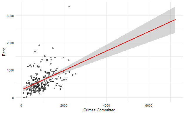
Check for correlation using Pearson’s Correlation Coefficient Test.

cor.test(alldatajoined_simple$n, alldatajoined_simple$estimate, method = "pearson")

Pearson’s product-moment correlation

data: alldatajoined_simple$n and alldatajoined_simple$estimate… t = 9.1764, df = 198, p-value < 2.2e-16… alternative hypothesis: true correlation is not equal to 0… 95 percent confidence interval: 0.4409235 0.6367331… sample estimates: cor 0.5462482

Analysis With Crimes Per Unit Area

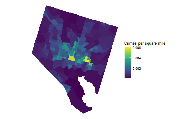
Mutate the data to add area of each tract. Use this column to define and add a crime per area column. Drop units in order to plot, but note what they were.

alldatajoined_perarea<-alldatajoined_simple %>% 
  mutate(area = st_area(.))%>%
  mutate(crimeperarea = (n/area))%>%
  drop_units()

#note that units are miles

Create a chloropleth map of crimes per square mile for each tract.

ggplot(alldatajoined_perarea, aes(fill = crimeperarea)) + 
  geom_sf(color = NA) + 
  scale_fill_viridis_c() + 
  theme_void() + 
  labs(fill = "Crimes per square mile")

Make a smoothed scatter plot of crimes per square mile versus rent.

ggplot(alldatajoined_perarea, aes(x = crimeperarea, y = estimate)) + 
  theme_minimal() + 
  geom_point(alpha = 0.5) + 
  geom_smooth(method = "lm", color = "red") +
  labs(x="Number of Crimes", y="Rent") 

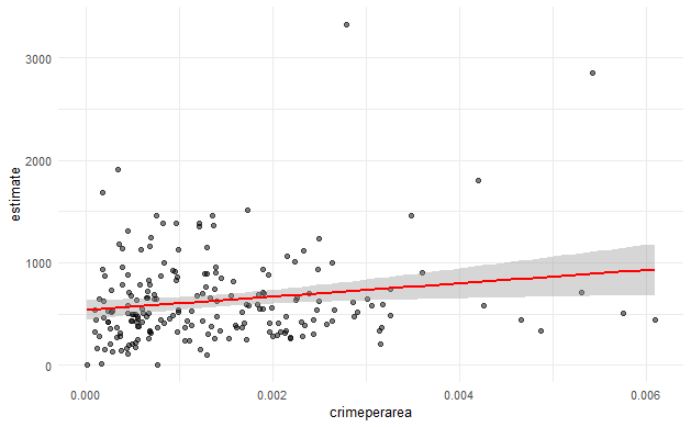
Check for correlation using Pearson’s Correlation Coefficient Test.

cor.test(alldatajoined_perarea$crimeperarea, alldatajoined_perarea$estimate, method = "pearson")

Pearson’s product-moment correlation

data: alldatajoined_perarea$crimeperarea and alldatajoined_perarea$estimate… t = 2.4798, df = 198, p-value = 0.01398… alternative hypothesis: true correlation is not equal to 0… 95 percent confidence interval: 0.03567281 0.30495286… sample estimates: cor 0.1735549

Discussion

I chose to test these relationships because I wanted to know how the amount of highly publicized crime affected housing prices for renters. I expected there to be a negative correlation between the two. I assumed in areas with more crime, landlords would be forced to decrease asking rent in order to find willing tenants, bringing down the average rent in that tract. Additionally, these serious crimes are the most well known as they get greater news coverage, so would more likely factor into a renter’s decision on a home. The results of this analysis, however, suggest a positive correlation between crime and rent. In hindsight, this makes sense because people are unlikely to commit crimes where they live.

An interesting aspect of these results is that area-wise crime rates had a less positive relationship with rent than did simple counts. Future analysis could factor in nearest neighbor crime counts, possibly with weighted regression, to get a more complete picture.